Consider to download this Jupyter Notebook and run locally, or test it with Colab.
In this notebook, we will look at density modeling with Gaussian mixture models (GMMs). In Gaussian mixture models, we describe the density of the data as \[
p(\boldsymbol x) = \sum_{k=1}^K \pi_k \mathcal{N}(\boldsymbol x|\boldsymbol \mu_k, \boldsymbol \Sigma_k)\,,\quad \pi_k \geq 0\,,\quad \sum_{k=1}^K\pi_k = 1
\]
The goal of this notebook is to get a better understanding of GMMs and to write some code for training GMMs using the EM algorithm. We provide a code skeleton and mark the bits and pieces that you need to implement yourself.
N_split =200# number of data points per mixture componentN = N_split*3# total number of data pointsx = []y = []for k inrange(3): x_tmp, y_tmp = np.random.multivariate_normal(m[k], S[k], N_split).T x = np.hstack([x, x_tmp]) y = np.hstack([y, y_tmp])data = np.vstack([x, y])
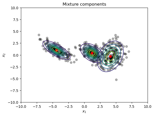
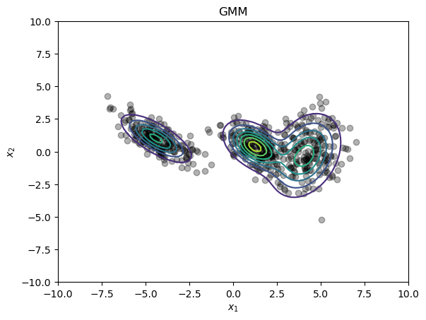
Visualization of the dataset
X, Y = np.meshgrid(np.linspace(-10,10,100), np.linspace(-10,10,100))pos = np.dstack((X, Y))mvn = multivariate_normal(m[0,:].ravel(), S[0,:,:])xx = mvn.pdf(pos)# plot the datasetplt.figure()plt.title("Mixture components")plt.plot(x, y, 'ko', alpha=0.3)plt.xlabel("$x_1$")plt.ylabel("$x_2$")# plot the individual components of the GMMplt.plot(m[:,0], m[:,1], 'or')for k inrange(3): mvn = multivariate_normal(m[k,:].ravel(), S[k,:,:]) xx = mvn.pdf(pos) plt.contour(X, Y, xx, alpha =1.0, zorder=10)# plot the GMMplt.figure()plt.title("GMM")plt.plot(x, y, 'ko', alpha=0.3)plt.xlabel("$x_1$")plt.ylabel("$x_2$")# build the GMMgmm =0for k inrange(3): mix_comp = multivariate_normal(m[k,:].ravel(), S[k,:,:]) gmm += w[k]*mix_comp.pdf(pos)plt.contour(X, Y, gmm, alpha =1.0, zorder=10);
Train the GMM via EM
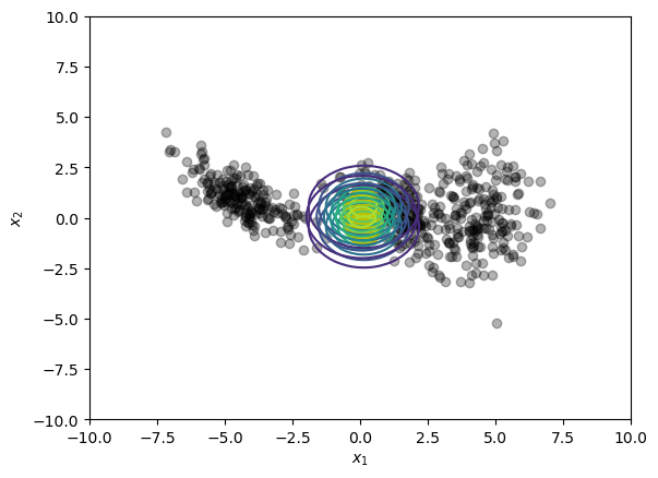
Initialize the parameters for EM
K =3# number of clustersmeans = np.zeros((K,2))covs = np.zeros((K,2,2))for k inrange(K): means[k] = np.random.normal(size=(2,)) covs[k] = np.eye(2)weights = np.ones((K,1))/Kprint("Initial mean vectors (one per row):\n"+str(means))
Initial mean vectors (one per row):
[[ 0.1252245  -0.42940554]
 [ 0.1222975   0.54329803]
 [ 0.04886007  0.04059169]]
#EDIT THIS FUNCTIONNLL = [] # log-likelihood of the GMMgmm_nll =0for k inrange(K): gmm_nll += weights[k]*multivariate_normal.pdf(mean=means[k,:], cov=covs[k,:,:], x=data.T)NLL += [-np.sum(np.log(gmm_nll))]plt.figure()plt.plot(x, y, 'ko', alpha=0.3)plt.plot(means[:,0], means[:,1], 'oy', markersize=25)for k inrange(K): rv = multivariate_normal(means[k,:], covs[k,:,:]) plt.contour(X, Y, rv.pdf(pos), alpha =1.0, zorder=10)plt.xlabel("$x_1$");plt.ylabel("$x_2$");
First, we define the responsibilities (which are updated in the E-step), given the model parameters \(\pi_k, \boldsymbol\mu_k, \boldsymbol\Sigma_k\) as \[
r_{nk} := \frac{\pi_k\mathcal N(\boldsymbol
x_n|\boldsymbol\mu_k,\boldsymbol\Sigma_k)}{\sum_{j=1}^K\pi_j\mathcal N(\boldsymbol
x_n|\boldsymbol \mu_j,\boldsymbol\Sigma_j)}
\]
Given the responsibilities we just defined, we can update the model parameters in the M-step as follows: \[\begin{align*}
\boldsymbol\mu_k^\text{new} &= \frac{1}{N_k}\sum_{n = 1}^Nr_{nk}\boldsymbol x_n\,,\\
\boldsymbol\Sigma_k^\text{new}&= \frac{1}{N_k}\sum_{n=1}^Nr_{nk}(\boldsymbol x_n-\boldsymbol\mu_k)(\boldsymbol x_n-\boldsymbol\mu_k)^\top\,,\\
\pi_k^\text{new} &= \frac{N_k}{N}
\end{align*}\] where \[
N_k := \sum_{n=1}^N r_{nk}
\]
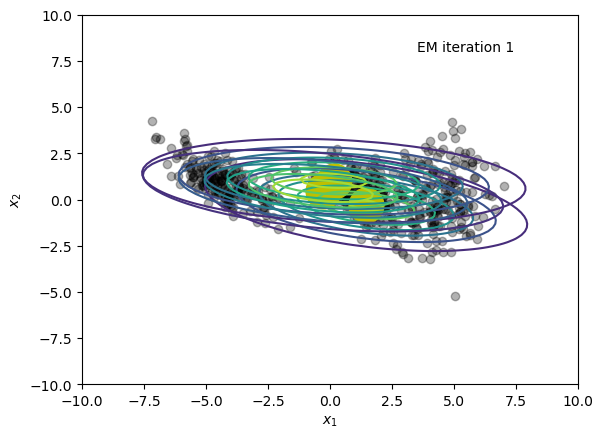
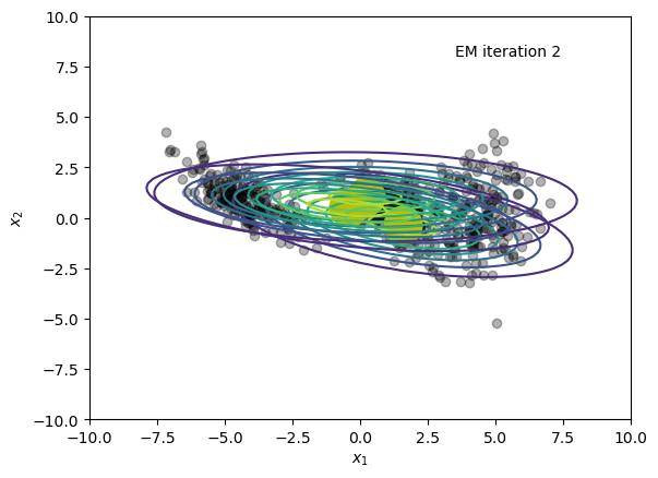
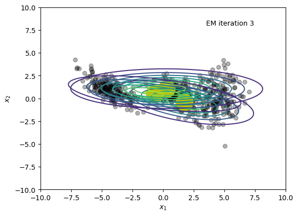
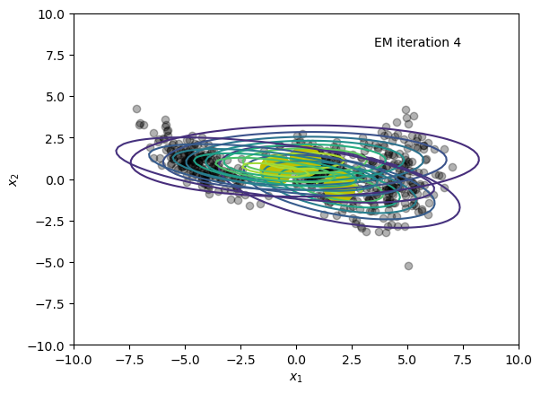
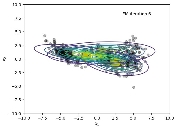
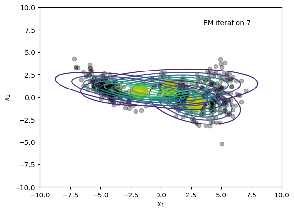
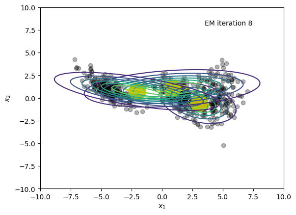
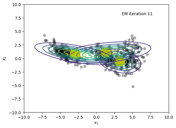
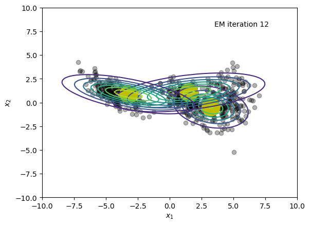
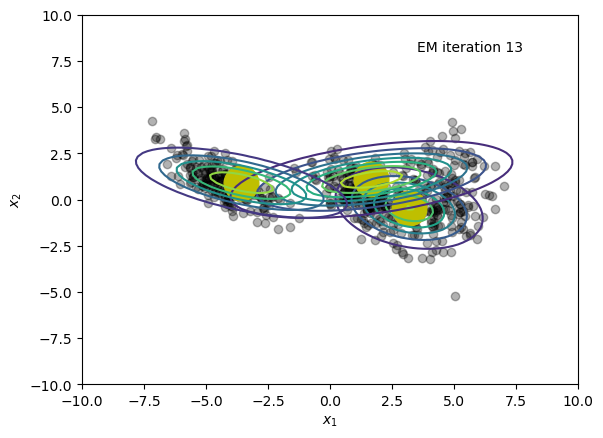
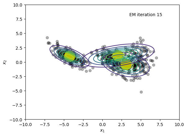
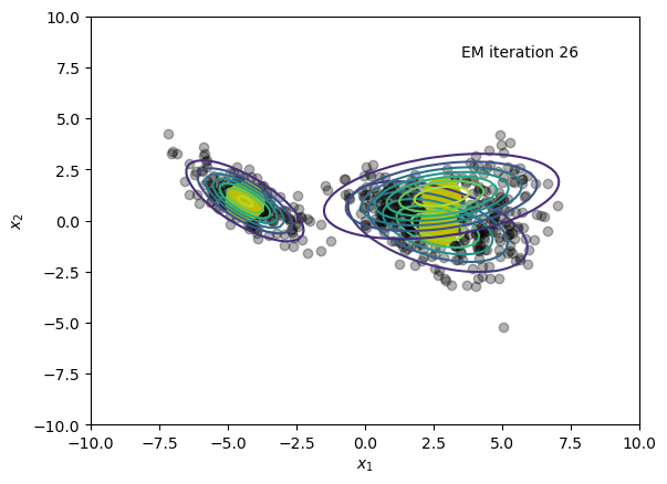
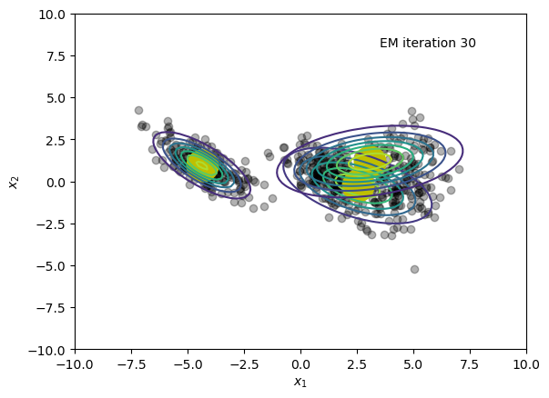
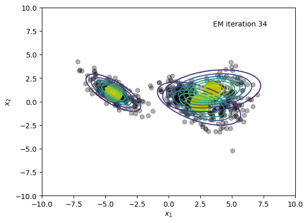
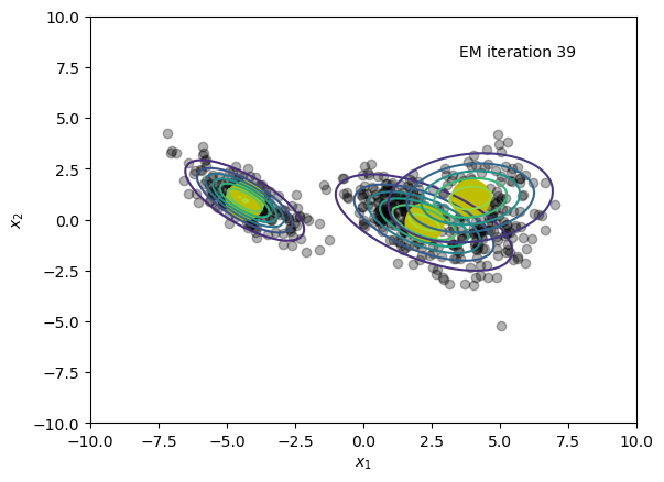
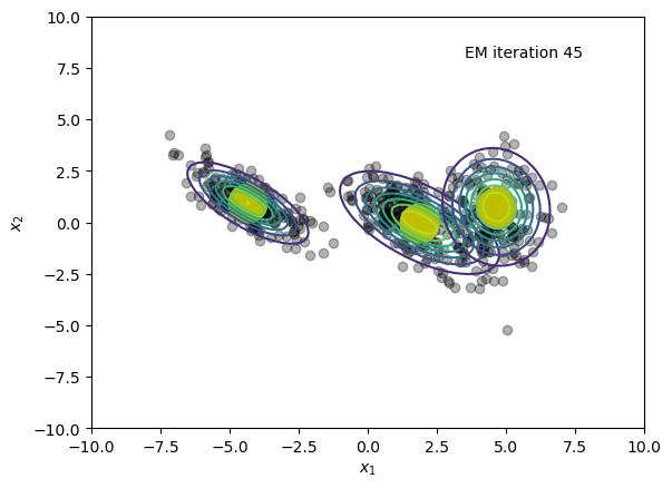
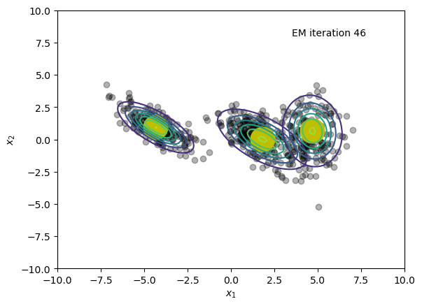
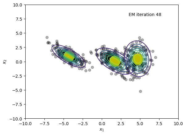
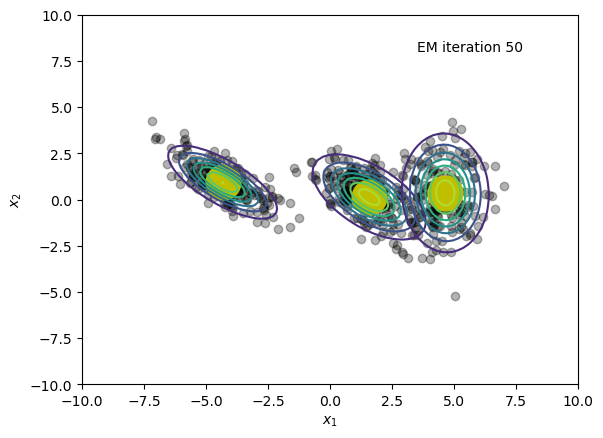
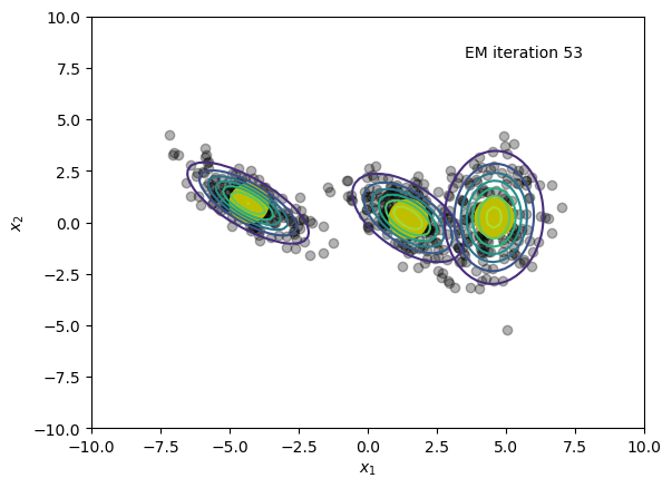
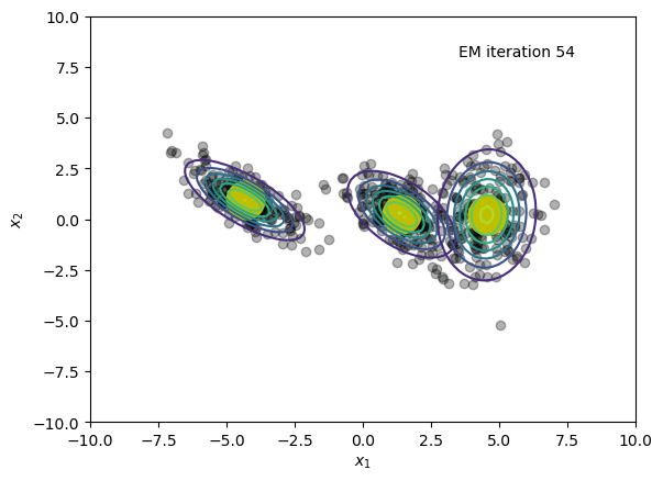
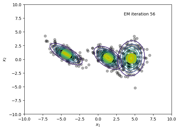
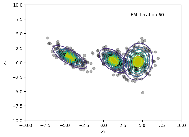
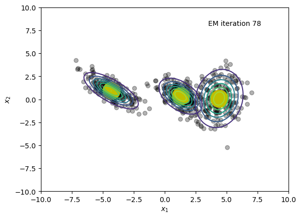
EM Algorithm
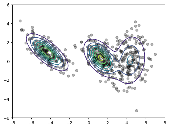
#EDIT THIS FUNCTIONr = np.zeros((K,N)) # will store the responsibilitiesfor em_iter inrange(100): means_old = means.copy()# E-step: update responsibilitiesfor k inrange(K): r[k] = weights[k]*multivariate_normal.pdf(mean=means[k,:], cov=covs[k,:,:], x=data.T) r = r/np.sum(r, axis=0)# M-step N_k = np.sum(r, axis=1)for k inrange(K):# update means means[k] = np.sum(r[k]*data, axis=1)/N_k[k]# update covariances diff = data - means[k:k+1].T _tmp = np.sqrt(r[k:k+1])*diff covs[k] = np.inner(_tmp, _tmp)/N_k[k]# weights weights = N_k/N# log-likelihood gmm_nll =0for k inrange(K): gmm_nll += weights[k]*multivariate_normal.pdf(mean=means[k,:].ravel(), cov=covs[k,:,:], x=data.T) NLL += [-np.sum(np.log(gmm_nll))] plt.figure() plt.plot(x, y, 'ko', alpha=0.3) plt.plot(means[:,0], means[:,1], 'oy', markersize=25)for k inrange(K): rv = multivariate_normal(means[k,:], covs[k]) plt.contour(X, Y, rv.pdf(pos), alpha =1.0, zorder=10) plt.xlabel("$x_1$") plt.ylabel("$x_2$") plt.text(x=3.5, y=8, s="EM iteration "+str(em_iter+1))if la.norm(NLL[em_iter+1]-NLL[em_iter]) <1e-6:print("Converged after iteration ", em_iter+1)break# plot final the mixture modelplt.figure()gmm =0for k inrange(3): mix_comp = multivariate_normal(means[k,:].ravel(), covs[k,:,:]) gmm += weights[k]*mix_comp.pdf(pos)plt.plot(x, y, 'ko', alpha=0.3)plt.contour(X, Y, gmm, alpha =1.0, zorder=10)plt.xlim([-8,8]);plt.ylim([-6,6]);plt.show()
/var/folders/nl/7_2jcxd12wb5z06jvsj1v4240000gn/T/ipykernel_39400/3431812709.py:34: RuntimeWarning: More than 20 figures have been opened. Figures created through the pyplot interface (`matplotlib.pyplot.figure`) are retained until explicitly closed and may consume too much memory. (To control this warning, see the rcParam `figure.max_open_warning`). Consider using `matplotlib.pyplot.close()`.
  plt.figure()
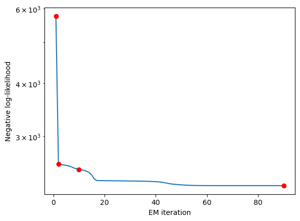
Converged after iteration 89
plt.figure()plt.semilogy(np.linspace(1,len(NLL), len(NLL)), NLL)plt.xlabel("EM iteration");plt.ylabel("Negative log-likelihood");idx = [0, 1, 9, em_iter+1]for i in idx: plt.plot(i+1, NLL[i], 'or')plt.show()